Learning Objectives
By the end of this lesson, you will be able to:
- Explain what cell formatting is and why it matters.
- Apply font styles, colors, fills, borders and cell styles.
- Align, wrap, merge, indent and rotate cell content.
- Apply number, currency, percentage and date formats.
- Use Format Painter, Clear Formatting and basic Conditional Formatting.
Lesson Overview
Data by itself is just numbers and words. Formatting is what turns a plain worksheet into a professional-looking report — clear headers, aligned numbers, easy-to-read fonts, sensible currency and percentage formats, and helpful colour cues. In this lesson you will learn every everyday formatting tool on the Excel Home tab, from font size to conditional formatting, with practical examples and shortcuts.
Introduction
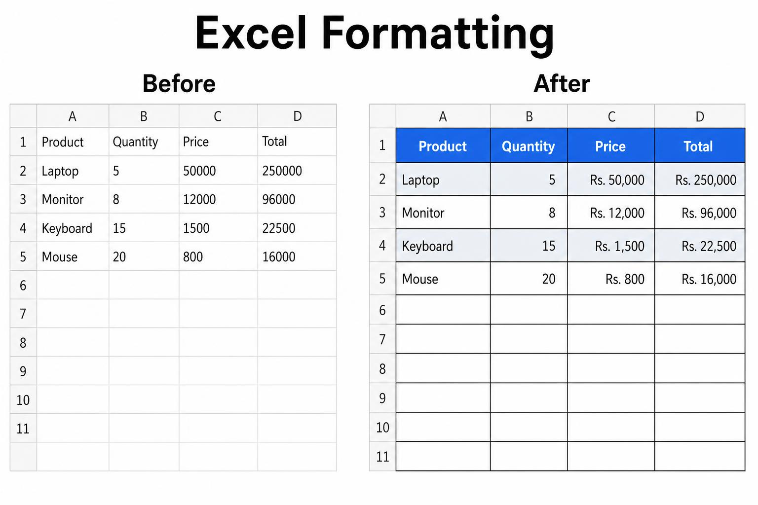
Imagine you receive an Excel file where every cell looks the same — no bold headers, no borders, prices without currency symbols, dates shown as numbers like 45680. It's hard to read, easy to misinterpret, and looks unfinished. Now imagine the same data with a bold header row, currency in ₹, right-aligned numbers, and green highlights for the top performers. Suddenly the report tells a story. That transformation — with zero change to the actual values — is cell formatting.
What is Cell Formatting?
Cell formatting is the way a cell's contents are displayed. It changes how a value looks — font, colour, size, borders, alignment, number style — without changing the actual value stored in the cell. The number 0.25 can be displayed as 0.25, 25%, or 25.00% depending on the format you apply, but Excel still uses 0.25 in every calculation.
Why Formatting Matters
Bold headers, aligned numbers and borders make data easy to scan.
A well-formatted sheet looks like a report, not a scratchpad.
Currency and date formats prevent misreading of numbers.
Colours and conditional formatting highlight what matters.
Font Formatting
Every font control lives on the Home tab → Font group. You can change the font name, size, style, colour and add underline — exactly like in Microsoft Word.
| Control | What it does | Shortcut |
|---|---|---|
| Font Name | Change the typeface (Calibri, Arial, Aptos, etc.) | — |
| Font Size | Make text bigger or smaller (default 11) | — |
| Bold | Emphasize text with heavier weight | Ctrl + B |
| Italic | Slanted text for notes or emphasis | Ctrl + I |
| Underline | Line under text — great for headings | Ctrl + U |
| Font Colour | Change the colour of the text (A with red bar) | — |
Fill Color & Borders
Fill Colour (the paint-bucket icon) changes the background of a cell. It's the fastest way to make header rows stand out or to group related cells.
Borders (the grid icon next to Fill Colour) draw lines around cells. Excel gridlines you see on screen do not print by default; borders do. Common choices are All Borders, Outside Borders and Thick Outside Borders.
Cell Styles
Cell Styles (Home tab → Styles group) are ready-made combinations of font, fill and border. One click applies a whole look — Title, Heading 1, Heading 2, Good, Bad, Neutral, Accent 1-6, Total, and more. They are consistent, fast and easy to update across a workbook.
Alignment
Alignment controls where the content sits inside a cell. Horizontal alignment can be Left, Center or Right. By default, Excel left-aligns text and right-aligns numbers — this is a helpful visual clue that a number is really stored as a number and not as text.
Vertical alignment — Top, Middle or Bottom — matters when the row is taller than a single line of text. For header rows with larger height, choose Middle alignment for a clean look.
Wrap Text & Merge
Wrap Text makes long text fit in a narrow column by breaking it into multiple lines within the same cell instead of spilling into the next column. Select the cell(s) and click Home → Wrap Text.
Merge & Center combines two or more selected cells into one and centres the content. It is perfect for titles that sit above a table. Use it sparingly — merged cells can make sorting, filtering and pivot tables misbehave.
Orientation & Indent
Text Orientation (the icon with the tilted ab) lets you rotate cell text — 90°, 45° or vertical. It is useful when column headers are long but the columns need to stay narrow, like in a comparison matrix.
Indent and Decrease Indent push text away from the left edge of the cell. Use them to create sub-levels in a list, e.g. main category on one row and its sub-items indented one level below.
Number Formats
Number formats change how a value looks — again, the underlying value never changes. You'll find the dropdown in Home → Number.
| Format | Underlying value | Displayed as |
|---|---|---|
| General | 1234.5 | 1234.5 (default, no special format) |
| Number | 1234.5 | 1,234.50 |
| Currency | 1234.5 | ₹1,234.50 / $1,234.50 |
| Accounting | 1234.5 | ₹ 1,234.50 (symbol aligned left) |
| Percentage | 0.25 | 25% |
| Date (Short) | 45680 | 19-Feb-2025 |
| Time | 0.75 | 6:00 PM |
| Text | 007 | 007 (kept as-is) |
Use Increase Decimal and Decrease Decimal (the two icons with arrows below the format dropdown) to control how many digits appear after the decimal point.
Format Painter
The Format Painter (paintbrush icon on the Home tab) copies formatting from one cell and applies it to another — no need to set fonts, colours and borders again. Select the source cell, click the brush, then click (or drag over) the target cells. Double-click the brush to paint multiple ranges; press Esc to stop.
Clear Formatting
To remove all formatting but keep the values, select the cells and go to Home → Editing → Clear → Clear Formats. This is far safer than deleting and retyping data when you just want to reset the look.
Conditional Formatting (Basic Introduction)
Conditional Formatting automatically formats cells based on their value — for example, colour every sale over ₹50,000 in green, or highlight duplicates in red. You'll find it on Home → Conditional Formatting. The most common beginner options are:
- Highlight Cells Rules — greater than, less than, between, duplicates, text contains.
- Top/Bottom Rules — top 10, bottom 10, above average.
- Data Bars — a mini in-cell bar chart based on value.
- Color Scales — heatmap colours from low to high.
- Icon Sets — arrows or traffic-light icons based on value.
Real-Life Example
You have a monthly sales report with columns Salesperson, Region, Target, Sales, Achievement %. In under two minutes you can:
- 1. Bold the header row and give it a green fill with white text.
- 2. Apply All Borders to the data range.
- 3. Format Target and Sales as Currency (₹).
- 4. Format Achievement % as Percentage with 0 decimals.
- 5. Add Conditional Formatting → Highlight Cells → Greater than 100% in green.
The same data now looks like a management report — with zero change to the underlying numbers.
Best Practices
- Use one font for the whole workbook (Calibri or Aptos work well).
- Keep header rows bold, filled and centred; keep data rows plain.
- Right-align numbers, left-align text, centre only headers.
- Use Cell Styles instead of manual formatting — easier to update later.
- Always apply a proper number format (currency, %, date) — never format cells as text for numbers.
- Use conditional formatting to highlight, not to decorate.
Common Mistakes
- Merging cells inside the data area — breaks sorting and filtering.
- Using too many colours and fonts — a report looks messy, not professional.
- Formatting numbers as Text — Excel then cannot SUM or AVERAGE them.
- Applying manual borders instead of using Cell Styles or a Table.
- Forgetting to remove formatting before pasting into a new sheet.
Keyboard Shortcuts
| Shortcut | What it does |
|---|---|
Ctrl + B | Bold |
Ctrl + I | Italic |
Ctrl + U | Underline |
Ctrl + 1 | Open Format Cells dialog |
Ctrl + Shift + $ | Apply Currency format |
Ctrl + Shift + % | Apply Percentage format |
Ctrl + Shift + # | Apply Date format |
Ctrl + Shift + ! | Apply Number format with thousand separator |
Alt + H, H | Open Fill Colour palette |
Alt + H, B | Open Borders menu |
Key Terms
How a cell's content is displayed — font, colour, borders, number style.
The background colour of a cell.
A visible line drawn around a cell that also prints.
A saved bundle of formatting you can apply in one click.
A rule that controls how a value is shown — currency, %, date, etc.
Tool that copies formatting from one range and pastes it on another.
Automatic formatting based on the value inside the cell.
Combines selected cells into one and centres the content.
Remember Box
Ctrl + 1 to open the full Format Cells dialog and unlock every option in one place.Practice Questions
- 1. Type a small sales table (Name, Sales, Target) and format the header row bold, white text on green fill, with All Borders.
- 2. Format the Sales column as Currency with 0 decimal places.
- 3. Add a new column Achievement % = Sales / Target and format it as Percentage.
- 4. Use Format Painter to copy the header row formatting to another table in the same sheet.
- 5. Apply Conditional Formatting to highlight cells greater than 100% in green.
Quick Quiz (MCQs)
Chapter Summary
- Cell formatting controls how data looks — never the value itself.
- The Home tab hosts font, fill, borders, alignment, number formats and styles.
- Cell Styles apply a consistent look in one click; use them over manual formatting.
- Number formats (Currency, Percentage, Date) prevent misreading of numbers.
- Format Painter copies formatting; Clear Formatting removes it while keeping values.
- Conditional Formatting highlights cells automatically based on rules.
- Good formatting = readable, professional, easy-to-scan reports.
Practice this lesson with real files
Get free practice workbooks, notes and doubt solving inside the free VIP WhatsApp community.
Join Free WhatsApp VIP Community